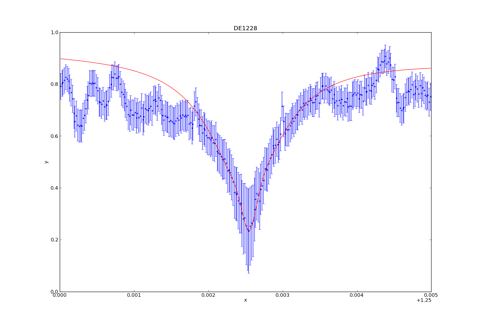
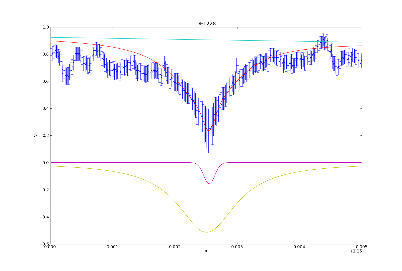
I have spent the last month or so immersing myself in Sherpa, the Python-built program I am using to make the measurements of the Potassium absorption line at 1.2525 microns. While finally coming up for air, I am going to share how I’ve used Sherpa in order to fit a model (or rather, 3 combined models) to the spectral feature so I can make the desired measurements. I will walk you through an example, the plotting and fitting of target “DE1228”.
To start, you need to have all of the data available. Using the BDNYC database developed last semester, we load into arrays the wavelength, flux, and snr values from may 30th, 2007:
>>> w = bdnyc.targets[33].nir[‘high’][‘NIRSPEC’][‘2007may30’][61][‘wl’]
>>> f = bdnyc.targets[33].nir[‘high’][‘NIRSPEC’][‘2007may30’][61][‘flux’]
>>> snr = bdnyc.targets[33].nir[‘high’][‘NIRSPEC’][‘2007may30’][61][‘snr’]
I then used a series of numpy commands to chop the arrays so as to only contain the values from 1.25 to 1.255 microns. Once that was done, I converted the snr to uncertainty values and stored them in an array called “unc”. Since these actions did not require Sherpa, I will omit them from this post. Once I had this completed, it was time to create the Sherpa data structure required for analysis. You use these commands:
>>> from sherpa.astro.ui import * # This is necessary if you are using Sherpa in a non-standalone version.
>>> data = unpack_arrays(w,f) # Loads the wavelength and flux arrays into the data structure, which I’ve originally named “data”.
>>> data.name = ‘DE1228’ # Give Sherpa the name of the target — this is not necessary, but it will automatically title any plots from now on.
Now that the data structure is created, we can now start using the sherpa functions to load in the data, models, uncertainties, etc. and bind them to an “id” number. These are the commands I used next:
>>> set_data(1, data) # I am using the id number “1”, which is the default id number, but I will explicitly state it so you can see how to state it.
>>> set_staterror(1, unc) # Load in uncertainties as the error
>>> plot_data(1) # This plots the data. Error is automatically plotted as well. This is not a necessary step for fitting, but it’s so you can see what you’re dealing with.
>>> set_source(1, powlaw1d.pl+gauss1d.g1+lorentz1d.l1) # I used a model containing a power law, gaussian profile, and lorentzian profile to fit the data and absorption line.
At this stage in the game, all of the data is now inputted, and now we have to play around. If you want to fit the models to the data, you have to use the fit command:
>>> fit(1)
If you do not prime the program by giving it some good values to start with, it may not come up with anything good. To prime, you can use:
>>> pl.ampl = 9
>>> l1. fwhm = 0.0011
Etcetera. You basically give somewhat good values to start with, and then have it fit the data from there. However, I wanted to fit to the peaks of the continuum data, and the fitting function seemed to be very unstable, often iving me horrible fits even when primed, so I was unable to find a good fit without manually fitting the models to the data myself. For DE1228, I used the values:
>>> pl.gamma = 10
>>> pl.ref = 1
>>> pl.ampl = 8.6
>>> l1.fwhm = 0.00115
>>> l1.pos = 1.25251
>>> l1.ampl = -0.00093
>>> g1.fwhm = 0.00021
>>> g1.pos = 1.25255
>>> g1.ampl = -0.157
Once you’ve fit the model to the data (either manually or not), you can plot the fit by typing:
>>> plot_fit(1)
You can then plot (or overplot) the different model components:
>>> plot_model_component(pl, overplot=True)
>>> plot_model_component(g1, overplot=True)
>>> plot_model_component(l1, overplot=True)
And that’s how I fit the models to the potassium absorption line. I’ve consolidated a lot of these numbers and commands into a table and python module (sherpa_tools.py). While specific, parts of the module can be applied to other people using Sherpa, so I can share the code if needed. In my next blog post, I’ll describe how to utilize the model to make the spectral line measurements (i.e. equivalent width, line-to-continuum flux ratio, full width half maximum).


I have also started using Sherpa recently, and while the capabilities are fantastic, the documentation is, well… less fantastic.
Right now I have seen on the ahelp web site that there should be a eqwidth() function, but when running it as an imported python module, I cannot seem to find it anywhere… Do you happen to know how to call it?
I know what you mean–the documentation is often very confusing.
When running Sherpa as an imported python module, if you want to utilize a Sherpa function you can find it in the sherpa.astro.ui module. So if you want to use eqwidth(), you can do:
>>> import sherpa.astro.ui as s_tools
>>> s_tools.eqwidth(continuum, continuum+line, … )
From what I can tell, all of the Sherpa functions are in the sherpa.astro.ui module. I’m hoping to write a blog entry in the next day or two about how I made spectral measurements, including the eqwidth, with Sherpa.
Hmm. Which version of Sherpa are you running? I am running 4.4.0 and cannot import the astro.ui module because of an internal import of a module that doesn’t to exist.
Just for those who may have found this in search of a problem to the import sherpa.astro.ui problem, I have posted a solution here: http://lusepuster.posterous.com/installing-sherpa-fitting-software-on-ubuntu – with kind and thankful thoughts to Kenny at the CXC help desk.
And yes, the dosumentation is very confusing – especially when trying to use Sherpa inside the script, in which case I would prefer to not use the .ui high-level commands that are designed for interactive use. But I haven’t gotten to be able to do that yet, unfortunately.
Interesting…I’m running 4.3.0, but I read the release notes of 4.4.0 and it didn’t mention changes in how to import it as a module. The only way I know how to run Sherpa as a Python module in a script is to import the ui commands.
To be honest, my Sherpa expertise is very limited, so I probably can’t help you troubleshoot the issue very well. However, CIAO has a helpdesk service (http://cxc.cfa.harvard.edu/helpdesk/) that helped me with Sherpa issues in the past, and it’s likely that they can help you out as well. If you go there and log in (you may have to set up an account), you can submit a ticket detailing the problem that you have and then someone on the team will help troubleshoot the issue (e.g. a module not working). Hope this helps!
Helpdesk was actually my next stop 🙂
And yep, so far I am (mostly) using the ui tools too, and then simply emptying the memory of all model components after the end of each run, but it’s a sort of dirty hack.
Pingback: Sherpa Part Three (Spectral Measurements) | BDNYC