BDNYC at AAS 225

BDNYC (and friends) are out in force for the 225th meeting of the American Astronomical Society!

Please come see our posters and talks (mostly on Monday). To whet your appetite, or if you missed them, here are some samplers:

Munazza Alam (Monday, 138.40)
High-Resolution Spectral Analysis of Red & Blue L Dwarfs
AAS225_Munazza_posterSara Camnasio (Monday, 138.39)
Multi-resolution Analysis of Red and Blue L Dwarfs
AAS225_Sara_posterKelle Cruz and Stephanie Douglas (Monday, 138.37)
When good fits go wrong: Untangling Physical Parameters of Warm Brown Dwarfs

AAS225_Stephanie_posterStephanie Douglas (Monday 138.19)
Rotation and Activity in Praesepe and the Hyades

AAS225_Steph_poster2Jackie Faherty (Talk, Monday 130.05)
Clouds in the Coldest Brown Dwarfs

Joe Filippazzo (Monday, 138.34)
Fundamental Parameters for an Age Calibrated Sequence of the Lowest Mass Stars to the Highest Mass Planets
Joe Filippazzo - AAS225

Paige Giorla (Monday, 138.44)
T Dwarf Model Fits for Spectral Standards at Low Spectral Resolution
AAS225_Paige_posterKay Hiranaka (Talk, Monday 130.04D)
Constraining the Properties of the Dust Haze in the Atmospheres of Young Brown Dwarfs

Erini Lambrides (Thursday, 432.02)
Can 3000 IR spectra unveil the connection between AGN and the interstellar medium of their host galaxies?

Emily Rice (Tuesday, 243.02)
STARtorialist: Astronomy Outreach via Fashion, Sci-Fi, & Pop Culture
AAS225_STARtorialistAdric Riedel (Monday, 138.38)
The Young and the Red: What we can learn from Young Brown Dwarfs
AAS225_Adric_poster

Ground Based Photometry

Here I want to calculate some photometric points from spectra for comparison with published values for a bunch of known brown dwarfs.

In order to get the true magnitude $$m$$ for an object, I first need to calculate the instrumental magnitude $$m_\text{inst}$$ and then correct for a number of effects. That is, I calculate the apparent magnitude from a particular place on the Earth and then add corrections to determine what it would be if we measured from space.

After all our corrections are made, the magnitude is given by:

$$!m=m_\text{inst}-ZP_m-k_m\cdot X$$

Instrumental Magnitude

The first term on the right in the equation above is the magnitude measured by the instrument on the ground, given by:

$$!m_\text{inst}=-2.5\log\left(\int f_\lambda (\lambda)\left(\frac{\lambda}{hc}\right)S_m(\lambda)d\lambda\right)$$

Where $$f_\lambda (\lambda)$$ is the energy flux density of the source in units of [erg s-1 cm-2 A-1] and $$S_m(\lambda)$$ is the scalar filter throughput for the band of interest.

Since I will be comparing my calculated magnitudes to photometry taken with photon counting devices, the factor of $$\frac{\lambda}{hc}$$ converts $$f_\lambda (\lambda)$$ to a photon flux density in units [photons s-1 cm-2 A-1].

Zero Point Correction

The second term in our magnitude equation is a first order correction to compare $$m_\text{inst}$$ to some standard we define as zero. I will use a flux calibrated spectrum of the A0 star Vega to calculate the zero point magnitude for the band:

$$!ZP_m=-2.5\log\left(\int f_{\lambda\text{ Vega}}(\lambda)\left(\frac{\lambda}{hc}\right)S_m(\lambda)d\lambda\right)$$

Just as we obtained our instrumental magnitude above.

Extinction Correction

The third term is to correct for the extinction of the source flux due to atmospheric absorption. We can get closer to the true apparent magnitude (above the atmosphere) by adding an extinction term:

$$!k_m\cdot\sec (z)=k_m\cdot X$$

Where $$k_m$$ is the extinction coefficient for the band of interest and $$\sec(z)=X$$ is the airmass.

The airmass is the optical path length of the atmosphere, which attenuates the source flux depending on its angle from the zenith $$z$$. Approximating the truly spherical atmosphere as plane-parallel, the airmass goes from $$X=1$$ at $$z=0^\circ$$ to $$X=2$$ at $$z=60^\circ$$. At zenith angles greater than that, the plane-parallel approximation falls apart and the airmass term gets complicated.

Where the airmass is the amount of atmosphere in the line of sight, the extinction coefficient is the amount by which the incident light is attenuated as it travels through the airmass. The extinction coefficient is related to the optical depth $$\tau$$ of the atmosphere as:

$$!m-m_0=-2.5\log\left(\frac{I}{I_0}\right)=-2.5\log (e^{-\tau X})=1.086\cdot\tau\cdot X=k_m\cdot X$$

Where $$m$$ and $$m_0$$ are the magnitudes below and above the atmosphere respectively.

Example: J21512543-2441000

As an example, I’d like to calculate the 2MASS J-band magnitude of the brown dwarf at 21h51m25.43s -24d41m00s given a low resolution NIR energy flux density from the SpeX Prism instrument on the 3m NASA Infrared Telescope Facility.

J21512543-2441000

Interpolating the filter throughput to the object spectrum and then integrating as in the equation above, I get $$J_\text{inst}=10.046$$ as my instrumental magnitude in the J-band.

Performing the same procedure on the flux calibrated spectrum of Vega, I get $$ZP_J=-5.721$$ for my J-band zero point magnitude.

Checking the FITS file header, I will use $$X=1.444625$$ for the airmass. The mean extinction coefficient for the MKO system J-band is given as $$k_J=0.0153$$ in Tokunaga & Vacca (2007), making the atmospheric correction term $$k_J\cdot X=0.0221$$.

The corrected magnitude is then:

$$!J=J_\text{inst}-ZP_J-k_J\cdot X=10.046-(-5.721)-0.0221=15.745$$

Which is only 0.007 magnitudes off from the value of $$J=15.752$$ from the 2MASS catalog.

Remaining Problems

As shown in the example above, this works… but not for every object.

2MASS apparent J magnitudes vs. my calculated apparent j magnitudes for 67 brown dwarfs. The solid black line is for perfect agreement and the dashed line is a best fit of the data.

2MASS apparent J magnitudes vs. my calculated apparent j magnitudes for 67 brown dwarfs. The solid black line is for perfect agreement and the dashed line is a best fit of the data.

2MASS apparent H magnitudes vs. my calculated apparent h magnitudes for 67 brown dwarfs. The solid black line is for perfect agreement and the dashed line is a best fit of the data.

2MASS apparent H magnitudes vs. my calculated apparent h magnitudes for 67 brown dwarfs. The solid black line is for perfect agreement and the dashed line is a best fit of the data.

I whittled down my sample of 875 to only those objects with flux units and airmass values taken at Mauna Kea so that I could use the same extinction coefficient and make sure they are all in the same units of [erg s-1 cm-2 A-1].

Then I pulled the 2MASS catalog J and H magnitudes with uncertainties for these remaining objects and plotted them against my calculated values with uncertainties.

To the left are the plots of the 67 objects that fit the selection criteria in J-band (above) and H-band (below).

Though it’s not the biggest sample, the deviation of the best fit line from unity suggests I’m off by a factor of 0.9 from the 2MASS catalog value across the board.

But more worrisome is the fact that most of the calculated magnitudes are not within the errors of the 2MASS magnitudes. This deviation ranges from very good agreement of a few thousandths of a magnitude up to the worst offenders of about 0.8 mags.

Filter Effective Wavelength(s)

The effective wavelength of a filter for narrow band photometry can easily be approximated by a constant and just looked up when needed. For broad band photometry, however, the width of the filter and the amount of flux in the band being measured actually come into play.

The effective wavelength of a filter is given by:

$$!\lambda_\text{eff}=\frac{\int \lambda \text{ }f_\lambda (\lambda)\text{ }S(\lambda)\text{ } d\lambda}{\int f_\lambda (\lambda)\text{ } S(\lambda)\text{ } d\lambda}$$

Where $$S(\lambda)$$ is the scalar filter throughput and $$f_\lambda$$ is the flux density in units of [erg s-1 cm-2 A-1] or [photons s-1 cm-2 A-1] depending upon whether you are using an energy measuring or a photon counting detector, respectively.

Here are the results for 67 brown dwarfs with complete spectrum coverage of the 2MASS J-band:

Effective wavelength values for the 2MASS J-band filter. Blue and green circles indicate lambda calculated using photon flux densities (PFD) and energy flux densities (EFD) respectively. Filled circles are for 67 confirmed brown dwarfs. Open circles are for Vega.

Effective wavelength values for the 2MASS J-band filter. Blue and green circles indicate lambda calculated using photon flux densities (PFD) and energy flux densities (EFD) respectively. Filled circles are for 67 confirmed brown dwarfs. Open circles are for Vega.

The red line on the plot shows the specified value given by 2MASS. For fainter objects like brown dwarfs (filled circles), the calculated effective wavelength of the J-band filter can shift redward by as much as 150 angstroms. Vega (open circles) shifts it blueward by about 30 angstroms.

The difference is small but measurable and demonstrates the dependence of the filter width, source spectrum, and detector type on the effective wavelength $$\lambda_\text{eff}$$ while doing broad band photometry.

Photon Flux Density vs. Energy Flux Density

One of the subtleties of photometry is the difference between magnitudes and colors calculated using energy flux densities (EFD) and photon flux densities (PFD).

The complication arises since the photometry presented by many surveys is calculated using PFD but spectra (specifically the synthetic variety) is given as EFD. The difference is small but measurable so let’s do it right.

The following is the process I used to remedy the situation by switching my models to PFD so they could be directly compared to the photometry from the surveys. Thanks to Mike Cushing for the guidance.

Filter Zero Points

Before we can calculate the magnitudes, we need filter zero points calculated from PFD. To do this, I started with a spectrum of Vega in units of [erg s-1 cm-2 A-1] snatched from STSci.

Then the zero point flux density in [photons s-1 cm-2 A-1] is:

$$!F_{zp}=\frac{\int p_V(\lambda) S(\lambda) d\lambda}{\int S(\lambda)d\lambda}=\frac{\int e_V(\lambda)\left( \frac{\lambda}{hc}\right) S(\lambda) d\lambda}{\int S(\lambda)d\lambda}$$

Where $$e_V$$ is the given energy flux density in [erg s-1 cm-2 A-1] of Vega, $$p_V$$ is the photon flux density in [photons s-1 cm-2 A-1], and $$S(\lambda)$$ is the scalar filter throughput.

Since I’m starting with a spectrum of Vega in EFD units, I need to multiply by $$\frac{\lambda}{hc}$$ to convert it to PFD units.

In Python, this looks like:

def zp_flux(band):
    from scipy import trapz, interp, log10
    (wave, flux), filt, h, c = vega(), get_filters()[band], 6.6260755E-27 # [erg*s], 2.998E14 # [um/s]
    I = interp(wave, filt['wav'], filt['rsr'], left=0, right=0)
    return trapz(I*flux*wave/(h*c), x=wave)/trapz(I, x=wave))

Calculating Magnitudes

Now that we have the filter zero points, we can calculate the magnitudes using:

$$!m = -2.5\log\left(\frac{F_\lambda}{F_{zp}}\right)$$

Where $$m$$ is the apparent magnitude and $$F_\lambda$$ is the flux from our source given similarly by:

$$!F_{\lambda}=\frac{\int p_\lambda(\lambda) S(\lambda) d\lambda}{\int S(\lambda)d\lambda}=\frac{\int e_\lambda(\lambda)\left( \frac{\lambda}{hc}\right) S(\lambda) d\lambda}{\int S(\lambda)d\lambda}$$

Since the synthetic spectra I’m using are given in EFD units, I need to multiply by $$\frac{\lambda}{hc}$$ to convert it to PFD units just as I did with my spectrum of Vega.

In Python the magnitudes are obtained the same way as above but we use the source spectrum in [erg s-1 cm-2 A-1] instead of Vega. Then the magnitude is just:

mag = -2.5*log10(source_flux(band)/zp_flux(band))

Below is an image that shows the discrepancy between using EFD and PFD to calculate colors for comparison with survey photometry.

The circles are colors calculated from synthetic spectra of low surface gravity (large circles) to high surface gravity (small circles). The grey lines are iso-temperature contours. The jumping shows the different results using PFD and EFD. The stationary blue stars, green squares and red triangles are catalog photometric points calculated from PFD.

The circles are colors calculated from synthetic spectra of low surface gravity (large circles) to high surface gravity (small circles). The grey lines are iso-temperature contours. The jumping shows the different results using PFD and EFD. The stationary blue stars, green squares and red triangles are catalog photometric points calculated from PFD.

Other Considerations

The discrepancy I get between the same color calculated from PFD and EFD though is as much as 0.244 mags (in r-W3 at 1050K), which seems excessive. The magnitude calculation reduces to:

$$!m = -2.5\log\left( \frac{\int e_\lambda(\lambda)S(\lambda) \lambda d\lambda}{\int e_V(\lambda) S(\lambda) \lambda d\lambda}\right)$$

Since the filter profile is interpolated with the spectrum before integration, I thought the discrepancy must be due only to the difference in resolution between the synthetic and Vega spectra. In other words, I have to make sure the wavelength arrays for Vega and the source are identical so the trapezoidal sums have the same width bins.

This reduces the discrepancy in r-W3 at 1050K from -0.244 mags to -0.067 mags, which is better. However, the discrepancy in H-[3.6] goes from 0.071 mags to -0.078 mags.

To Recapitulate

In summary, I had a spectrum of Vega and some synthetic spectra all in energy flux density units of [erg s-1 cm-2 A-1] and some photometric points from the survey catalogs calculated from photon flux density units of [photons s-1 cm-2 A-1].

In order to compare apples to apples, I first converted my spectra to PFD by multiplying by $$\frac{\lambda}{hc}$$ at each wavelength point before integrating to calculate my zero points and magnitudes.

Colors Diagnostic of Surface Gravity

The goal here is to find a prescription of colors diagnostic of brown dwarf surface gravity. Since early optical as well as far infrared spectra and photometry are uncommon, the bands of interest should only include i and z from SDSS; J, H and Ks from 2MASS; and W1, W2 and W3 (but not W4 with only 10 percent detection) from WISE.

In order to find said prescriptions, I used the BT-Settl models (at solar metallicity ranging from 1000 – 3000 K in effective temperature and 3.0 – 5.5 dex in log surface gravity) to produce a suite of color-color and color-parameter plots.

One method I employed was to choose one effective temperature (in this case 2500K) and anchor the colors in one band that doesn’t vary much between high and low surface gravity, e.g. z-band. Then I chose the other two bands by one that was more luminous at low gravity and one that was more luminous at high gravity, e.g. W2- and J-band respectively.

BT-Settl model spectra at 2500K

Then the color-color plot of these bands looks like:

In this plot of z-J vs. z-W2 the smallest circles are objects with high surface gravity and the largest have low surface gravity (log(g) = 5.5 to 3.5 respectively). The light grey lines are iso-temperature contours.

In this plot of z-J vs. z-W2 the smallest circles are objects with high surface gravity and the largest have low surface gravity (log(g) = 5.5 to 3.5 respectively). The light grey lines are iso-temperature contours.

In this particular case, there is little-to-no dispersion in z-J for Teff = 2500K (d = 0.009) and an appreciable dispersion in z-W2 for that same Teff (d = 0.32). Notice the tight vertical grouping (z-J) and dispersed horizontal grouping (z-W2) for the model objects of Teff = 2500K and varying log(g) in the red rectangle on the color-color plot above.

Double-checking with the color-Teff plots, we can see that the dispersion in z-J in the plot on the left is tiny and the horizontal offset in the color-color plot is due to the 0.32 magnitude dispersion in z-W2 on the right below.

Of course this is just a different way of looking at the same thing, but I might be able to find colors that are reliable indicators of gravity (and thus age) if I can find a bunch of these examples where the flux in the secondary and tertiary bands are flipped.

Of note is the fact that at this temperature in this color-color plot the points are also isolated, i.e. there are no degeneracies with objects of any other temperature. That means that if I find an object with a z-J = 1.65 or so, I know that it has an effective temperature of about 2500K. Then I can determine its age by seeing if its z-W2 color is closer to 3.3 (young) or 2.9 (old).

This of course does not work for all temperatures, as shown in the red circle in the color-color plot above. This demonstrates a degeneracy among hotter young objects (Teff = 3000K, log(g) = 3.5) and cooler old objects (Teff = 2800K, log(g) = 5.5) with a temperature difference of 200K.

Though there is no definitive combination of colors to identify the age of an object irrespective of temperature, what I have done here is found a collection of prescriptions that are reliable indicators of age over small temperature ranges.

Color vs. Spectral Type Model Comparison

Here are color vs. spectral type plots for the 2MASS J, H and Ks bands.

The blue circles are for the objects with parallax measurements. The red squares are for the AMES-Dusty model spectra with spectral types gleaned from effective temperature according to Golimowski et al (2004).

While the AMES-Dusty models are known not to be a good fit for objects with effective temperatures lower than about 2200K (shown by the disagreement in L dwarf colors of objects and models), the M dwarfs fit fairly well for J-Ks versus Spectral Type.

However, the models are under-luminous in J-H and over-luminous in H-Ks for M dwarfs, indicating a possible problem with H-band modeling. The models shown are calculated with a surface gravity of 5.5, which means that the models produce a “peakier” H-band than the objects actually exhibit.

In a color-color plot of J-H versus H-Ks, the H-band throws off the model colors on both axes causing a diagonal shift (bluer in J-H, redder in H-Ks) of M and L dwarfs compared to the models:

Identifying Nearby Young Stars, Part 1: Young Star Isochrones

As stars form, their position on the HR diagram (or, equivalently, a Color-Magnitude diagram) changes.   They start out very cool but physically very large and very bright; as they collapse under gravity and become fully supported by hydrogen fusion power, they become smaller and dimmer.

The practical upshot of all of this is that we can determine the ages of stars based on their HR diagram locations – for a given luminosity and color, there is an associated age.  This is particularly useful for low-mass objects, which take extremely long times to reach the main sequence: An M0 star probably takes 200 Myr to reach the main sequence (Dotter et al. 2008), while a brown dwarf will never reach any kind of main sequence, and will slowly cool and dim forever.

Typically, people use theoretical stellar evolution models like Baraffe et al. (1998), but in practice it is also possible to make empirical relations from known young stars with parallaxes, by fitting polynomials to them.  The diagram below shows a set of fifth-order (x5) polynomials that were fit to the single-star members of nearby young associations, as they appeared in Riedel et al. (2011).

A color-magnitude diagram of nearby young low-mass stars

A Color-magnitude diagram (Absolute V magnitude versus V-K photometric color) of M dwarf stars with parallaxes. The main sequence is represented by stars with trigonometric (annual) parallaxes within 10 parsecs of the Sun. M dwarf members of associations that are less than ~100 Myr old and closer than 100 parsecs are represented as colored and shaped items on the plot, and empirical isochrones are also shown.

As expected, we see multi-magnitude differences in the luminosity of Epsilon Chameleon members (pink) versus similarly-colored members of TW Hydra (yellow) or Beta Pictoris (blue).  On this basis, I presumed the nearby M dwarf AP Columbae was probably older than Beta Pictoris, but younger than AB Doradus (which annoyingly lies within the range of high-metallicity main sequence stars).

Of course, these polynomials are not perfect – they are dependent on the quality of the parallaxes and whether a star actually is a single, “normal” member of the group… and the polynomials are only useful between the boundaries for which there is data to fit.  As of the time when I made these polynomial fits, there were only two young brown dwarfs — both members of TW Hydra — with parallaxes AND Johnson V photometry, which is why all the other lines terminate at the middle and hotter M spectral types.  If I replaced the Johnson V colors with something redder (I or J-band) it would be a lot easier to produce empirical isochrones for brown dwarfs… although at the moment, extremely few young brown dwarfs are known.

Spectral Energy Distributions

The goal here was to investigate the atmospheric properties of known young objects and identify new brown dwarf candidates by producing extended spectral energy distributions (SEDs).

These SEDs are constructed by combining WISE mid-infrared photometry with our extensive database of optical and near-infrared spectra and parallaxes. The BDNYC Database has about 875 objects and the number of objects with parallaxes is about 250.

My code queries the database and the parallax measurements by right ascension and declination and then identifies the matches with enough spectra and photometry to produce an SED. Next, it checks the flux and wavelength units and makes the appropriate conversions to [ergs][s-1][cm-2][cm-1] and [um] respectively.

It then runs a fitting routine across BT-Settl models of every permutation of:

  • 400 K < Teff < 4500 K in 50 K increments,
  • 3.0 dex < log(g) < 5.5 dex in 0.1 dex increments, and
  • 0.5 MJup < radius < 1.3 MJup in 0.05 MJup increments.

Once the best match is found, it plots the synthetic spectrum (grey) along with the photometric points converted to flux in each SDSS, 2MASS and WISE bands (grey dots). In this manner, the fitting routine guesses the effective temperature, surface gravity and radius simultaneously.

Here are some preliminary plots:

Brown Dwarf Synthetic Photometry

The goal here was to get the synthetic colors in the SDSS, 2MASS and WISE filters of ~2000 model objects generated by the PHOENIX stellar and planetary atmosphere software.

Since it would be silly (and incredibly slow… and much more boring) to just calculate and store every single color for all 12 filter profiles, I wrote a module to calculate colors a la carte.

The Filters

I got the J, H, and K band relative spectral response (RSR) curves in the 2MASS documentation, the u, g, r, i and z bands from the SDSS documentation, and the W1, W2, W3, and W4 bands from the WISE documentation.

I dumped all my .txt filter files into one directory and wrote a function to grab them all, pull out the wavelength and transmission values, and output the filter name in position [0], x-values in [1], and y-values in [2]:

def get_filters(filter_directory):
  import glob, os
  files = glob.glob(filter_directory+'*.txt')
 
  if len(files) == 0:
    print 'No filters in', filter_directory
  else:
    filter_names = [os.path.splitext(os.path.basename(i))[0] for i in files]
    RSR = [open(i) for i in files]
    filt_data = [filter(None,[map(float,i.split()) for i in j if not i.startswith('#')]) for j in RSR]
    for i in RSR: i.close()
 
    RSR_x = [[x[0] for x in i] for i in filt_data]
    RSR_y = [[y[1] for y in i] for i in filt_data]
    filters = {}
    for i,j,k in zip(filter_names,RSR_x,RSR_y):
      filters[i] = j, k, center(i)
 
    return filters

Calculating Apparent Magnitudes

We can’t have colors without magnitudes so here’s a function to grab the Teff and log g specified spectra, and calculate the apparent magnitudes in a particular band:

def mags(band, teff='', logg='', bin=1):
  from scipy.io.idl import readsav
  from collections import Counter
  from scipy import trapz, log10, interp
  
  s = readsav(path+'modelspeclowresdustywise.save')
  Fr, Wr = [i for i in s.modelspec['fsyn']], [i for i in s['wsyn']]
  Tr, Gr = [int(i) for i in s.modelspec['teff']], [round(i,1) for i in s.modelspec['logg']]
  
  # The band to compute
  RSR_x, RSR_y, lambda_eff = get_filters(path)[band]
  
  # Option to specify an effective temperature value
  if teff:
    t = [i for i, x in enumerate(s.modelspec['teff']) if x == teff]
    if len(t) == 0:
      print "No such effective temperature! Please choose from 1400K to 4500K in 50K increments or leave blank to select all."
  else:
    t = range(len(s.modelspec['teff']))
  
  # Option to specify a surfave gravity value
  if logg:
    g = [i for i, x in enumerate(s.modelspec['logg']) if x == logg]
    if len(g) == 0:
      print "No such surface gravity! Please choose from 3.0 to 6.0 in 0.1 increments or leave blank to select all."
  else:
    g = range(len(s.modelspec['logg']))
  
  # Pulls out objects that fit criteria above
  obj = list((Counter(t) & Counter(g)).elements())
  F = [Fr[i][::bin] for i in obj]
  T = [Tr[i] for i in obj]
  G = [Gr[i] for i in obj]
  W = Wr[::bin]
  
  # Interpolate to find new filter y-values
  I = interp(W,RSR_x,RSR_y,left=0,right=0)
  
  # Convolve the interpolated flux with each filter (FxR = RxF)
  FxR = [convolution(i,I) for i in F]
  
  # Integral of RSR curve over all lambda
  R0 = trapz(I,x=W)
  
  # Integrate to find the spectral flux density per unit wavelength [ergs][s-1][cm-2] then divide by R0 to get [erg][s-1][cm-2][cm-1]
  F_lambda = [trapz(y,x=W)/R0 for y in FxR]
  
  # Calculate apparent magnitude of each spectrum in each filter band
  Mags = [round(-2.5*log10(m/F_lambda_0(band)),3) for m in F_lambda]
  
  result = sorted(zip(Mags, T, G, F, I, FxR), key=itemgetter(1,2))
  result.insert(0,W)
  
  return result

Calculating Colors

Now we can calculate the colors. Next, I wrote a function to accept any two bands with options to specify a surface gravity and/or effective temperature as well as a bin size to cut down on computation. Here’s the code:

def colors(first, second, teff='', logg='', bin=1):
  (Mags_a, T, G) = [[i[j] for i in get_mags(first, teff=teff, logg=logg, bin=bin)[1:]] for j in range(3)]
  Mags_b = [i[0] for i in get_mags(second, teff=teff, logg=logg, bin=bin)[1:]]
  colors = [round(a-b,3) for a,b in zip(Mags_a,Mags_b)]
  
  print_mags(first, colors, T, G, second=second)
  
  return [colors, T, G]

The PHOENIX code gives the flux as Fλ in cgs units [erg][s-1][cm-2][cm-1] but as long as both spectra are in the same units the colors will be the same.

Makin’ It Handsome

Then I wrote a short function to print out the magnitudes or colors in the Terminal:

def print_mags(first, Mags, T, G, second=''):
  LAYOUT = "{!s:10} {!s:10} {!s:25}"
  
  if second:
    print LAYOUT.format("Teff", "log g", first+'-'+second)
  else:
    print LAYOUT.format("Teff", "log g", first)
  
  for i,j,k in sorted(zip(T, G, Mags)):
    print LAYOUT.format(i, j, k)

The Output

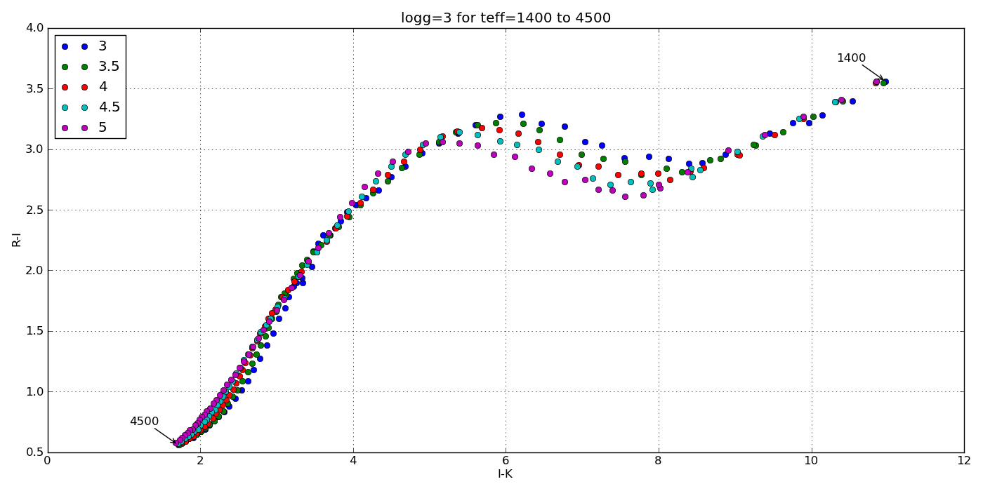
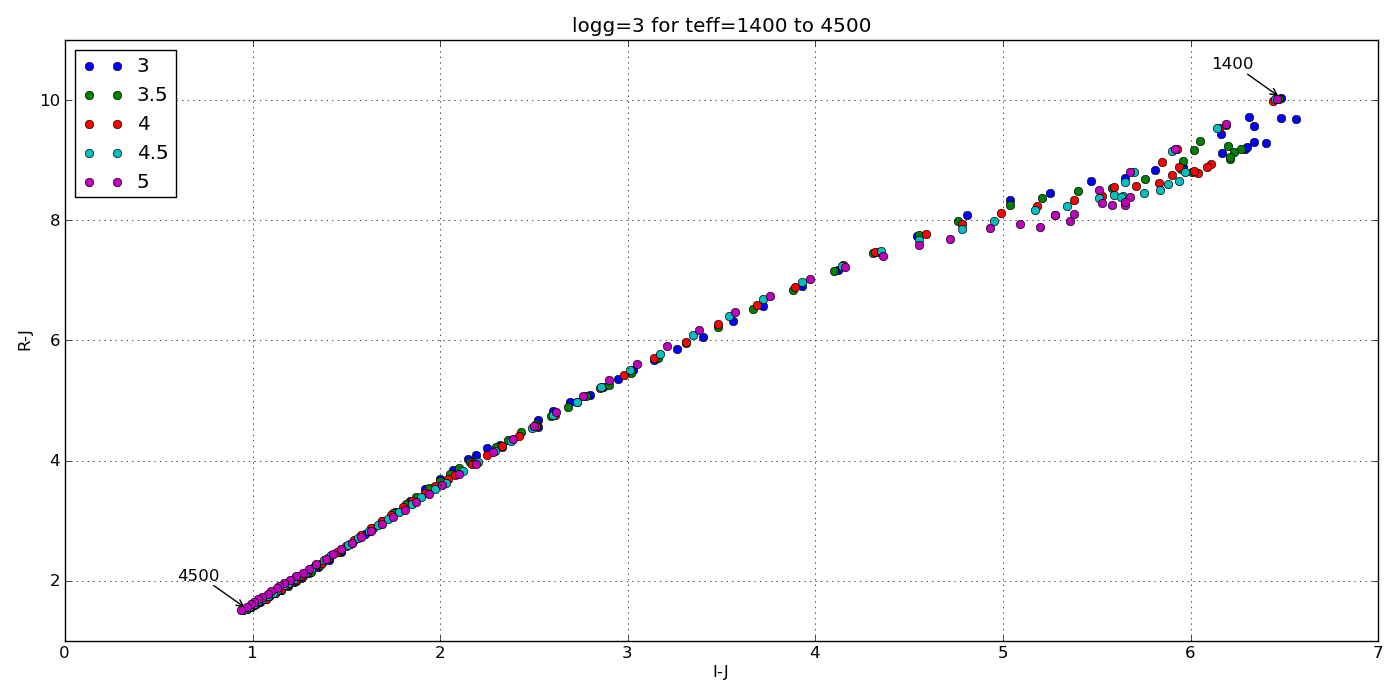
Then if I just want the J-K color for objects with log g = 4.0 over the entire range of effective temperatures, I launch ipython and just do:

In [1]: import syn_phot as s
In [2]: s.colors('J','K', logg=4)
Teff -------- log g -------- J-K
1400.0 ------ 4.0 ---------- 4.386
1450.0 ------ 4.0 ---------- 4.154
...
4450.0 ------ 4.0 ---------- 0.756
4500.0 ------ 4.0 ---------- 0.733

Similarly, I can specify just the target effective temperature and get the whole range of surface gravities. Or I can specify an effective temperature AND a specific gravity to get the color of just that one object with:

In [3]: s.colors('i','W2', teff=3050, logg=5)
Teff -------- log g -------- J-K
3050.0 ------ 5.0 ---------- 3.442

I can also reduce the number of data points in each flux array if my sample is very large. I just have to specify the number of data points to skip with the “bin” optional parameter. For example:

In [4]: s.colors('W1','W2', teff=1850, bin=3)

This will calculate the W1-W2 color for all the objects with Teff = 1850K and all gravities, but only take every third flux value.

I also wrote functions to generate color-color, color-parameter and color-magnitude plots but those will be in a different post.

Plots!

Here are a few color-parameter animated plots I made using my code. Here’s how I made them. Click to animate!

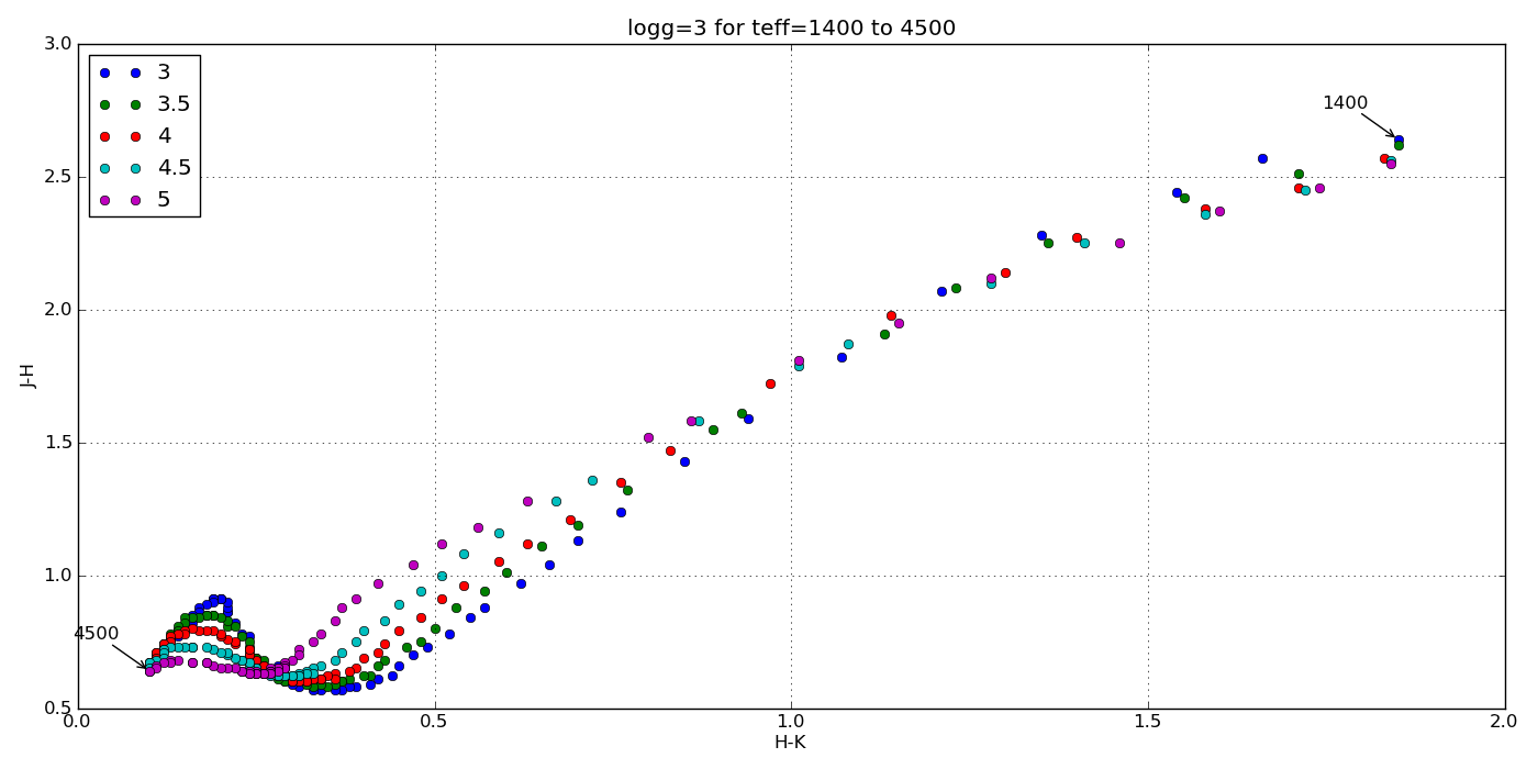
And here are a few colorful-colorful color-color plots I made:

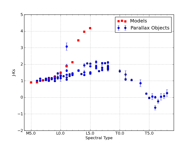
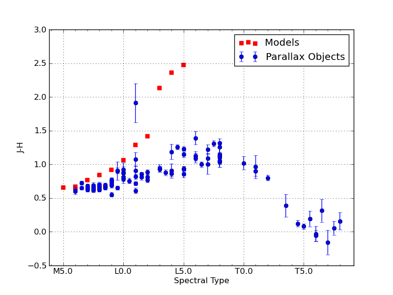
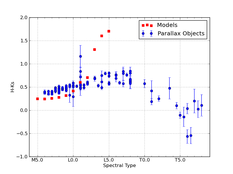
Plots with observational data

Just to be sure I’m on base, here’s a color-color plot of J-H vs. H-Ks for objects with a log surface gravity of 5 dex (blue dots) plotted over some data for the Chamaeleon I Molecular Cloud (semi-transparent) from Carpenter et al. (2002).

The color scale is for main sequence stars and the black dots are probable members of the group. Cooler dwarfs move up and to the right.

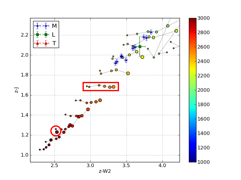
And here’s a plot of J-Ks vs. z-Ks as well as J-Ks vs. z-J. Again, the blue dots are from my synthetic photometry code at log(g)=5 and the semi-transparent points with errors are from Dahn et al. (2002).