Determining ages for brown dwarfs is one of the trickiest aspects in our research, yet a very important one as they allow us to estimate masses. One way many researchers estimate ages is by attempting to match the motions of the object to that of stellar moving groups with known ages. A match in XYZ-UVW space can suggest membership which would imply the brown dwarf is coeval with that group. One can calculate XYZ positions and UVW velocities in Python or your favorite programming language. BDNYC is now hosting a stellar kinematics web application that can do this for you.
Category Archives: Python
AstrodbWeb
Followers of this blog and our team’s scientific endeavors may know we have a curated database of brown dwarfs we work with. An initial version of this database has been published in Filippazzo et al. 2015 and contains information for 198 objects. The database is also maintained on Github, where we welcome contributions from other researchers. We’ve developed a set of tools for astronomers to work with SQL databases, namely the Python package astrodbkit. This package can be applied to other SQL databases allowing astronomers from all fields of research to manage their data.
Here we introduce a new tool: AstrodbWeb, a web-based interface to explore the BDNYC database.
Continue reading
Documentation using Sphinx
Reply
Sphinx is a free, online tool that helps generate documentation for primarily Python projects. We use it for HTML format outputs, but it also supports LaTeX, ePub, Texinfo, manual pages, and plain text formats. The markup language of Sphinx is reStructuredText (reST) (for documentation see http://sphinx-doc.org/rest.html). Of Sphinx’s many features, the one most useful thus far is its auto-documentation of Python files, the steps of which this post details below.
Sphinx auto-documentation steps:
- Install Sphinx at the command line using:
easy_install -U Sphinx - Read through the Sphinx documentation at http://sphinx-doc.org/.
- Run Sphinx’s Getting Started function
Sphinx-quickstartto quickly set up directories and configurations. NOTE: Since I have already completed this setup, it DOES NOT need to be run again for the BDNYC documentation.- Access the documentation directories in Dropbox through the shared folder BDNYCdb/Documentation
- The Documentation folder contains the .rst and .py files that Sphinx uses to build documentation. Place any files for which documentation is to be made within that directory since Sphinx automatically looks there.
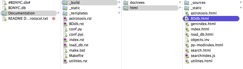 BDdb.html within the Documentation directories
- The index.rst file is the master file that contains the table of contents (known as a TOCtree) for the entire documentation. Within the TOCtree, Sphinx knows that all the files are .rst, so there is no need to specify the file extension or path. The index also serves as a welcome page for users, so it may include an introduction or other information that would be useful for outside reference. Within the TOCtree (and all of reST) indentation and notation is especially important. Below is an example of a functioning TOCtree.
.. toctree::

:maxdepth: 2

# blank line

BDdb

utilities

astrotools

load_db

Database_instructions
The “maxdepth” function specifies the depth of nesting allowed. In order to keep the index clean and aesthetically simple, a maximum of one nested page is reasonable. In other files, however, highly nested pages are not only common, but well-supported by reST.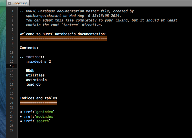
- Screenshot of index.rst
- For each item in the TOCtree of the index file, there must be a corresponding .rst file in the main directory for Sphinx to nest within the index HTML file. In the above example, a Database_instructions.rst file might contain in plain English how to interact with the database, while the BDdb.rst file contains the auto-documentation of BDdb.py.
- The .rst file within the TOCtree of the index must be formatted like below to correctly call for the Python files.
[name of module]

================    # make page header (see http://sphinx-doc.org/rest.html)

.. automodule:: [name of Python file w/o extension]

:members:    # tells Sphinx to pull from the file

# blank line

:undoc-members:

:show-inheritance: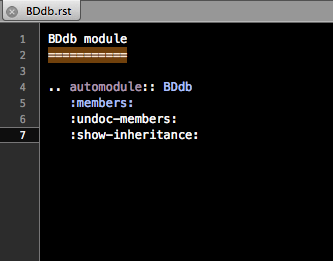
Screenshot of BDdb.rst
- The referenced Python files for auto-documentation can either be in located in the main directory, or their location can be specified. Since we will be constantly pushing and pulling from Github, it is best for those doing documentation to change the file path to their local copy of BDdb.py, astrotools.py, etc, before making documentation. This can be achieved as follows:
- Open conf.py, which is the configuration file for Sphinx. It was produced during the “quickstart” function to allow easy modifications of aesthetic features (i.e., theme, font), and facilitate the HTML building process.
- Change the file path in line 21 to the applicable local copy.
- Comment out the file path of previous users in order to make it easier for others to update documentation.
- In order to make the HTML files, move Terminal to the directory of the documentation, i.e., ‘…/Dropbox/BDNYCdb/Documentation’ and run
make html.- The
make htmlfunction comes build-in through running “quickstart” and uses the makefile in the main directory. It can take other functions as well, includingmake clean, which deletes the entire contents of the “build” directory. - Sphinx should put the generated HTML files in the /_build/html directory.
- The
- To make the HTML files live on BDNYC.org/database, use the application Cyberduck, which can be downloaded at http://cyberduck.en.softonic.com/mac.
- Click “Open Connection” and put in the server, username, and password.
- Drag and drop any .rst and HTML files that were modified into the appropriate directory and the documentation should go live immediately!
References:
http://sphinx-doc.org/ — Sphinx documentation homepage
http://sphinx-doc.org/contents.html — Outline of Sphinx documentation
http://sphinx-doc.org/rest.html — Using reStructuredText in Sphinx
http://sphinx-doc.org/ext/autodoc.html — Auto-documentation documentation
http://cyberduck.en.softonic.com/mac — Download Cyberduck
Setting Up Your BDNYC Astro Python Environment
Here’s a step-by-step tutorial on how to set up your Python development environment.
Distribution and Compiler
The first step is to install Anaconda. Click here, select the appropriate version for your machine and operating system, download the .dmg file, open it and double-click the installer.
Make sure that when the installer asks where to put the distribution, you choose your actual hard drive and not some sub-directory on your machine. This will make things much easier later on.
What’s nice about this distribution is that it includes common plotting, computing, and astronomy packages such as numpy and scipy, astropy, matplotlib, and many others.
Next you’ll need a C compiler. If you’re using MacOSX, I recommend using Xcode which you can download free here. (This step may take a while so go get a beverage.) Once the download is complete, run the installer.
Required Packages
For future installation of packages, I recommend using Pip. To install this, at your Terminal command line type sudo easy_install pip. Then whenever you want to install a package you might need, you just open Terminal and do pip install package_name.
Not every package is this easy (though most are). If you can’t get something through Pip just download, unzip and put the folder of your new module with the rest of your packages in the directory /anaconda/pkgs/.
Then in Terminal, navigate to that directory with cd /anaconda/pkgs/package_dir_name and do python setup.py install.
Development Tools
MacOSX comes with the text editing application TextEdit but it is not good for editing code. I strongly recommend using TextMate though it is not free so you should ask your advisor to buy a license for you! Otherwise, some folks find the free TextWrangler to be pretty good.
Next, you’ll want to get access to the BDNYC database. Detailed instructions are here on how to setup Dropbox and Github on your machine in order to interact with the database.
Launching Python
Now to use Python, in Terminal just type ipython --pylab. I recommend always launching Python this way to have the plotting library preloaded.
Enjoy!
BDNYC Database Setup
WARNING: The information on this is outdated. We recommend looking into the up-to-date documentation at trac (internal) and ReadTheDocs.
Read this post first if your development environment needs setting up. Then…
Setting Up the Database
To install the database, open a Terminal session and do:
pip install BDNYCdb
Then download the public database file BDNCY198.db here or get the unpublished BDNYC.db file from Dropbox. (Ask a group member for the invite!)
Accessing the Database
Now you can load the entire database into a Python variable simply by launching the Python interpreter and pointing the get_db() function to the database file by doing:
In [1]: from BDNYCdb import BDdb

In [2]: db = BDdb.get_db('/path/to/your/Dropbox/BDNYCdb/BDNYC.db')
Voila!
In the database, each source has a unique identifier (or ‘primary key’ in SQL speak). To see an inventory of all data for one of these sources, just do:
In [3]: db.inventory(id)
where id is the source_id.
Now that you have the database at your fingertips, you’ll want to get some info out of it. To do this, you can use SQL queries.
Here is a detailed post about how to write an SQL query.
Further documentation for sqlite3 can be found here. Most commands involve wrapping SQL language inside python functions. The main method we will use to fetch data from the database is list():
In [5]: data = db.list( "SQL_query_goes_here" ).fetchall()
Example Queries
Some SQL query examples to put in the command above (wrapped in quotes of course):
- SELECT shortname, ra, dec FROM sources WHERE (222<ra AND ra<232) AND (5<dec AND dec<15)
- SELECT band, magnitude, magnitude_unc FROM photometry WHERE source_id=58
- SELECT source_id, band, magnitude FROM photometry WHERE band=’z’ AND magnitude<15
- SELECT wavelength, flux, unc FROM spectra WHERE observation_id=75”
As you hopefully gathered:
- Returns the shortname, ra and dec of all objects in a 10 square degree patch of sky centered at RA = 227, DEC = 10
- Returns all the photometry and uncertainties available for object 58
- Returns all objects and z magnitudes with z less than 15
- Returns the wavelength, flux and uncertainty arrays for all spectra of object 75
The above examples are for querying individual tables only. We can query from multiple tables at the same time with the JOIN command like so:
- SELECT t.name, p.band, p.magnitude, p.magnitude_unc FROM telescopes as t JOIN photometry AS p ON p.telescope_id=t.id WHERE p.source_id=58
- SELECT p1.magnitude-p2.magnitude FROM photometry AS p1 JOIN photometry AS p2 ON p1.source_id=p2.source_id WHERE p1.band=’J’ AND p2.band=’H’
- SELECT src.designation, src.unum, spt.spectral_type FROM sources AS src JOIN spectral_types AS spt ON spt.source_id=src.id WHERE spt.spectral_type>=10 AND spt.spectral_type<20 AND spt.regime=’optical’
- SELECT s.unum, p.parallax, p.parallax_unc, p.publication_id FROM sources as s JOIN parallaxes AS p ON p.source_id=s.id
As you may have gathered:
- Returns the survey, band and magnitude for all photometry of source 58
- Returns the J-H color for every object
- Returns the designation, U-number and optical spectral type for all L dwarfs
- Returns the parallax measurements and publications for all sources
Alternative Output
As shown above, the result of a SQL query is typically a list of tuples where we can use the indices to print the values. For example, this source’s g-band magnitude:
In [9]: data = db.list("SELECT band,magnitude FROM photometry WHERE source_id=58").fetchall()

In [10]: data

Out[10]: [('u', 25.70623),('g', 25.54734),('r', 23.514),('i', 21.20863),('z', 18.0104)]

In [11]: data[1][1]

Out[11]: 25.54734
However we can also query the database a little bit differently so that the fields and records are returned as a dictionary. Instead of db.query.execute() we can do db.dict() like this:
In [12]: data = db.dict("SELECT * FROM photometry WHERE source_id=58").fetchall()

In [13]: data

Out[13]: [<sqlite3.Row at 0x107798450>, <sqlite3.Row at 0x107798410>, <sqlite3.Row at 0x107798430>, <sqlite3.Row at 0x1077983d0>, <sqlite3.Row at 0x1077982f0>]

In [14]: data[1]['magnitude']

Out[14]: 25.54734
Database Schema and Browsing
In order to write the SQL queries above you of course need to know what the names of the tables and fields in the database are. One way to do this is:
In [15]: db.list("SELECT sql FROM sqlite_master").fetchall()
This will print a list of each table, the possible fields, and the data type (e.g. TEXT, INTEGER, ARRAY) for that field.
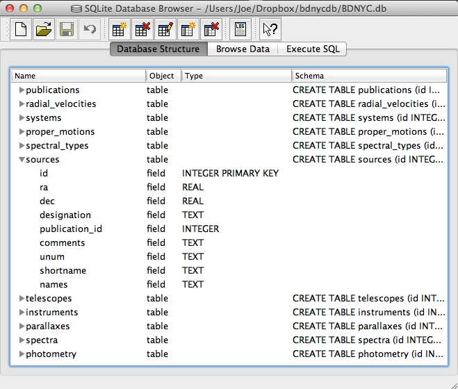 Even easier is to use the DB Browser for SQLite pictured at left which lets you expand and collapse each table, sort and order columns, and other fun stuff.
It even allows you to manually create/edit/destroy records with a very nice GUI.
IMPORTANT: If you are using the private database keep in mind that if you change a database record, you immediately change it for everyone since we share the same database file on Dropbox. Be careful!
Always check and double-check that you are entering the correct data for the correct source before you save any changes with the SQLite Database Browser.
SQL Queries
An SQL database is comprised of a bunch of tables (kind of like a spreadsheet) that have fields (column names) and records (rows of data). For example, our database might have a table called students that looks like this:
| id | first | last | grade | GPA |
|---|---|---|---|---|
| 1 | Al | Einstein | 6 | 2.7 |
| 2 | Annie | Cannon | 6 | 3.8 |
| 3 | Artie | Eddington | 8 | 3.2 |
| 4 | Carlie | Herschel | 8 | 3.2 |
So in our students table, the fields are [id, first, last, grade, GPA], and there are a total of four records, each with a required yet arbitrary id in the first column.
To pull these records out, we tell SQL to SELECT values for the following fields FROM a certain table. In SQL this looks like:
In [1]: db.execute("SELECT id, first, last, grade, GPA FROM students").fetchall()

Out[1]: [(1,'Al','Einstein',6,2.7),(2,'Annie','Cannon',6,3.8),(3,'Artie','Eddington',8,3.2),(4,'Carlie','Herschel',8,3.2)]
Or equivalently, we can just use a wildcard “*” if we want to return all fields with the SQL query "SELECT * FROM students".
We can modify our SQL query to change the order of fields or only return certain ones as well. For example:
In [2]: db.execute("SELECT last, first, GPA FROM students").fetchall()

Out[1]: [('Einstein','Al',2.7),('Cannon','Annie',3.8),('Eddington','Artie',3.2),('Herschel','Carlie',3.2)]
Now that we know how to get records from tables, we can restrict which records it returns with the WHERE statement:
In [3]: db.execute("SELECT last, first, GPA FROM students WHERE GPA>3.1").fetchall()

Out[3]: [('Cannon','Annie',3.8),('Eddington','Artie',3.2),('Herschel','Carlie',3.2)]
Notice the first student had a GPA less than 3.1 so he was omitted from the result.
Now let’s say we have a second table called quizzes which is a table of every quiz grade for all students that looks like this:
| id | student_id | quiz_number | score |
|---|---|---|---|
| 1 | 1 | 3 | 89 |
| 2 | 2 | 3 | 96 |
| 3 | 3 | 3 | 94 |
| 4 | 4 | 3 | 92 |
| 5 | 1 | 4 | 78 |
| 6 | 3 | 4 | 88 |
| 7 | 4 | 4 | 91 |
Now if we want to see only Al’s grades, we have to JOIN the tables ON some condition. In this case, we want to tell SQL that the student_id (not the id) in the quizzes table should match the id in the students table (since only those grades are Al’s). This looks like:
In [4]: db.execute("SELECT quizzes.quiz_number, quizzes.score FROM quizzes JOIN students ON students.id=quizzes.student_id WHERE students.last='Einstein'").fetchall()

Out[4]: [(3,89),(4,78)]
So students.id=quizzes.student_id associates each quiz with a student from the students table and students.last='Einstein' specifies that we only want the grades from the student with last name Einstein.
Similarly, we can see who scored 90 or greater on which quiz with:
In [5]: db.execute("SELECT students.last, quizzes.quiz_number, quizzes.score FROM quizzes JOIN students ON students.id=quizzes.student_id WHERE quizzes.score>=90").fetchall()

Out[5]: [('Cannon',3,96),('Eddington',3,94),('Herschel',3,92),('Herschel',4,91)]
That’s it! We can JOIN as many tables as we want with as many restrictions we need to pull out data in the desired form.
This is powerful, but the queries can become lengthy. A slight shortcut is to use the AS statement to assign a table to a variable (e.g. students => s, quizzes => q) like such:
In [6]: db.execute("SELECT s.last, q.quiz_number, q.score FROM quizzes AS q JOIN students AS s ON s.id=q.student_id WHERE q.score>=90").fetchall()

Out[6]: [('Cannon',3,96),('Eddington',3,94),('Herschel',3,92),('Herschel',4,91)]
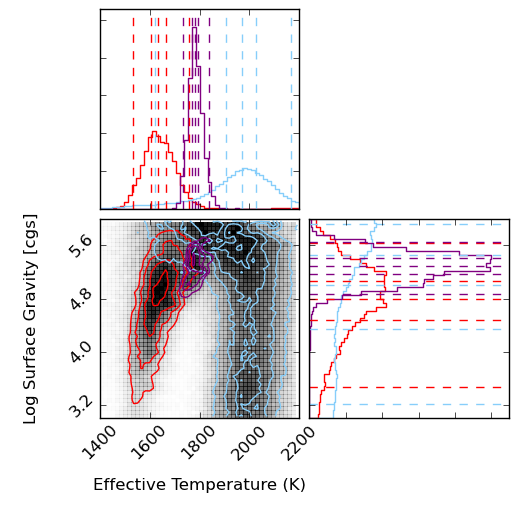
Visualizing results from low-res NIR spectral fits
In my first serious foray into Python and github I adapted some plotting code from Dan Foreman_Mackey with the help of Adrian Price-Whelan and Joe Filippazzo to create contour plots and histograms of my fitting results! These are histograms MCMC results for model fits to a low-resolution near-infrared spectrum of a young L5 brown dwarf, in temperature and gravity atmospheric parameters. The colors represent different segments of the spectrum – purple is YJH, blue is YJ, red is H. The take-away is that different segments of the spectrum results in different temperatures, and all parts of the spectrum make it look old (high gravity). This is probably because the overly-simplistic dust treatments in the models are not sufficient for young, low-mass objects.
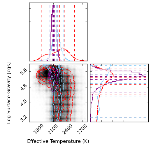
The baseline for comparison is the result for a field L5 dwarf, shown below. The temperatures are much more consistent with one another and what you would expect for an L5 spectral type from other methods, and the gravities are similarly high (although too high for comfort for J band). This is reassuring for the method in general and probably means that we need most sophisticated dust treatments in the models to handle giant-exoplanet-like young brown dwarfs. Paper will be submitted soon!
Photon Flux Density vs. Energy Flux Density
One of the subtleties of photometry is the difference between magnitudes and colors calculated using energy flux densities (EFD) and photon flux densities (PFD).
The complication arises since the photometry presented by many surveys is calculated using PFD but spectra (specifically the synthetic variety) is given as EFD. The difference is small but measurable so let’s do it right.
The following is the process I used to remedy the situation by switching my models to PFD so they could be directly compared to the photometry from the surveys. Thanks to Mike Cushing for the guidance.
Filter Zero Points
Before we can calculate the magnitudes, we need filter zero points calculated from PFD. To do this, I started with a spectrum of Vega in units of [erg s-1 cm-2 A-1] snatched from STSci.
Then the zero point flux density in [photons s-1 cm-2 A-1] is:
$$!F_{zp}=\frac{\int p_V(\lambda) S(\lambda) d\lambda}{\int S(\lambda)d\lambda}=\frac{\int e_V(\lambda)\left( \frac{\lambda}{hc}\right) S(\lambda) d\lambda}{\int S(\lambda)d\lambda}$$
Where $$e_V$$ is the given energy flux density in [erg s-1 cm-2 A-1] of Vega, $$p_V$$ is the photon flux density in [photons s-1 cm-2 A-1], and $$S(\lambda)$$ is the scalar filter throughput.
Since I’m starting with a spectrum of Vega in EFD units, I need to multiply by $$\frac{\lambda}{hc}$$ to convert it to PFD units.
In Python, this looks like:
def zp_flux(band):

    from scipy import trapz, interp, log10

    (wave, flux), filt, h, c = vega(), get_filters()[band], 6.6260755E-27 # [erg*s], 2.998E14 # [um/s]

    I = interp(wave, filt['wav'], filt['rsr'], left=0, right=0)

    return trapz(I*flux*wave/(h*c), x=wave)/trapz(I, x=wave))
Calculating Magnitudes
Now that we have the filter zero points, we can calculate the magnitudes using:
$$!m = -2.5\log\left(\frac{F_\lambda}{F_{zp}}\right)$$
Where $$m$$ is the apparent magnitude and $$F_\lambda$$ is the flux from our source given similarly by:
$$!F_{\lambda}=\frac{\int p_\lambda(\lambda) S(\lambda) d\lambda}{\int S(\lambda)d\lambda}=\frac{\int e_\lambda(\lambda)\left( \frac{\lambda}{hc}\right) S(\lambda) d\lambda}{\int S(\lambda)d\lambda}$$
Since the synthetic spectra I’m using are given in EFD units, I need to multiply by $$\frac{\lambda}{hc}$$ to convert it to PFD units just as I did with my spectrum of Vega.
In Python the magnitudes are obtained the same way as above but we use the source spectrum in [erg s-1 cm-2 A-1] instead of Vega. Then the magnitude is just:
mag = -2.5*log10(source_flux(band)/zp_flux(band))
Below is an image that shows the discrepancy between using EFD and PFD to calculate colors for comparison with survey photometry.
The circles are colors calculated from synthetic spectra of low surface gravity (large circles) to high surface gravity (small circles). The grey lines are iso-temperature contours. The jumping shows the different results using PFD and EFD. The stationary blue stars, green squares and red triangles are catalog photometric points calculated from PFD.
Other Considerations
The discrepancy I get between the same color calculated from PFD and EFD though is as much as 0.244 mags (in r-W3 at 1050K), which seems excessive. The magnitude calculation reduces to:
$$!m = -2.5\log\left( \frac{\int e_\lambda(\lambda)S(\lambda) \lambda d\lambda}{\int e_V(\lambda) S(\lambda) \lambda d\lambda}\right)$$
Since the filter profile is interpolated with the spectrum before integration, I thought the discrepancy must be due only to the difference in resolution between the synthetic and Vega spectra. In other words, I have to make sure the wavelength arrays for Vega and the source are identical so the trapezoidal sums have the same width bins.
This reduces the discrepancy in r-W3 at 1050K from -0.244 mags to -0.067 mags, which is better. However, the discrepancy in H-[3.6] goes from 0.071 mags to -0.078 mags.
To Recapitulate
In summary, I had a spectrum of Vega and some synthetic spectra all in energy flux density units of [erg s-1 cm-2 A-1] and some photometric points from the survey catalogs calculated from photon flux density units of [photons s-1 cm-2 A-1].
In order to compare apples to apples, I first converted my spectra to PFD by multiplying by $$\frac{\lambda}{hc}$$ at each wavelength point before integrating to calculate my zero points and magnitudes.
Memory Leaks in Python
I just spent a few hours tracking down a massive memory leak in the Python code I’m working on for my current project. Running the code on even a single object would eat up 4 GB of memory in my computer, and that slowed the entire system down to the point that other programs were unusable, even if they didn’t crash outright. After fixing the memory leak, the memory usage stayed between 200-204 MB for the entire time the program was running.
As it turns out, the problem was that every loop was creating several plots, and (even though I was writing them to files) not closing them with a plt.clf() except after the end of the loop, which only affected the last plot object.
The gist of it is, there are only a few reasons for memory leaks in Python.
- There’s some object you are opening (repeatedly) but not closing.
- You are repeatedly adding data to a list/dict and not removing the old data. (for instance, if you’re appending data to an array instead of replacing the array)
- There’s a memory leak in one of the libraries you’re calling. (unlikely)
source: http://www.lshift.net/blog/2008/11/14/tracing-python-memory-leaks
I haven’t successfully tried the methods listed in the above link (they seem to be for heavier-duty programming than we use) but that first reason is likely to be a problem for BDNYC: We open plot figures, we open the BDNYC database, we open .fits files with astropy… remember to close things properly.
For the record, this seems to be the correct sequence for making a matplotlib plot:
fig = pyplot.figure(1)
ax = fig.add_subplot(111) # or fig.add_axes()
ax.plot(<blah>)
ax.set_xlabel(<label>)
(...)
fig.savefig(<filename>)
fig.clf()
pyplot.close()
That last line was completely new to me, but is apparently necessary if you do it this way. Matplotlib works without creating a figure, adding axes to a figure, and then adding plot commands to the axis… but if used this way, you can actually edit multiple figures and their subplots at the same time — just specify which axis variable you want to add the plot element to. To my knowledge, this is a clear advantage over IDL: IDL can only operate on one plot at a time; trying to open a new one closes the old one.
Converting Between Decimal Degrees and Hours, Minutes, Seconds
Here’s a quick Python snippet I wrote to convert right ascension in decimal degrees to hours, minutes, seconds and declination to (+/-)degrees, minutes, seconds.
def deg2HMS(ra='', dec='', round=False):

  RA, DEC, rs, ds = '', '', '', ''

  if dec:

    if str(dec)[0] == '-':

      ds, dec = '-', abs(dec)

    deg = int(dec)

    decM = abs(int((dec-deg)*60))

    if round:

      decS = int((abs((dec-deg)*60)-decM)*60)

    else:

      decS = (abs((dec-deg)*60)-decM)*60

    DEC = '{0}{1} {2} {3}'.format(ds, deg, decM, decS)


  if ra:

    if str(ra)[0] == '-':

      rs, ra = '-', abs(ra)

    raH = int(ra/15)

    raM = int(((ra/15)-raH)*60)

    if round:

      raS = int(((((ra/15)-raH)*60)-raM)*60)

    else:

      raS = ((((ra/15)-raH)*60)-raM)*60

    RA = '{0}{1} {2} {3}'.format(rs, raH, raM, raS)


  if ra and dec:

    return (RA, DEC)

  else:

    return RA or DEC
For example:
In [1]: f.deg2HMS(ra=66.918277)

Out[1]: '4 27 40.386'
Or even:
In [2]: f.deg2HMS(dec=24.622590)

Out[2]: '+24 37 21.324'
Or if you want to round the seconds, just do:
In [3]: f.deg2HMS(dec=24.622590,round=True)

Out[3]: '+24 37 21'
And to convert hours, minutes and seconds into decimal degrees, we have:
def HMS2deg(ra='', dec=''):

  RA, DEC, rs, ds = '', '', 1, 1

  if dec:

    D, M, S = [float(i) for i in dec.split()]

    if str(D)[0] == '-':

      ds, D = -1, abs(D)

    deg = D + (M/60) + (S/3600)

    DEC = '{0}'.format(deg*ds)


  if ra:

    H, M, S = [float(i) for i in ra.split()]

    if str(H)[0] == '-':

      rs, H = -1, abs(H)

    deg = (H*15) + (M/4) + (S/240)

    RA = '{0}'.format(deg*rs)


  if ra and dec:

    return (RA, DEC)

  else:

    return RA or DEC
So we can get back our decimal degrees with:
In [4]: f.HMS2deg(ra='4 27 40.386', dec='+24 37 21.324')

Out[4]: (66.918, 24.622)